Force Multipliers Don’t Care
Large language models have accelerated the speed at which you can create messes by orders of magnitude. A pipeline that took months to prototype now takes a day. A classification system that required a team now takes one person with an API key. These tools are force multipliers, and force multipliers do not care what they multiply. They amplify good design and bad design equally.
You can prototype a pipeline in a day. You can also scale a broken pipeline in a day. Parallelization, batching, and automation are amplifiers. Before you reach for them, you need to know whether you are amplifying a solution or amplifying a problem. This chapter teaches the engineering discipline that makes the difference: how to design pipelines that run fast, fail gracefully, and survive the model changes that are coming whether you plan for them or not.
The LLM as Bottleneck Node
In any processing pipeline, something is the constraint. In LLM workflows, it is almost always the API call: rate limits (requests per minute, tokens per minute), latency per call, and context window size. Everything else, file I/O, JSON parsing, result aggregation, is fast by comparison.
You cannot make the LLM call faster. You do not control the provider’s infrastructure. You design the pipeline to maximize useful work within the constraints the provider imposes. This is the fundamental insight of this chapter: design around the bottleneck, not through it.
The first decision is whether your task is parallel or serial. The question is task independence: can each item be processed without knowledge of any other item’s result?
If yes, parallelize. Most classification, coding, and extraction tasks are embarrassingly parallel. Each record is independent. The model does not need to know what it said about the previous record to classify the current one. Send them all at once, up to your rate limit.
If items depend on prior results, serialize. Generator-critic loops (Chapter 5) are inherently serial: the critic’s output feeds back to the generator. Multi-turn refinement requires sequential processing. Arbitration that references prior judgments has ordering constraints.
Know which shape your task has before designing the pipeline. Getting this wrong in either direction costs you: parallelizing a serial task produces incorrect results; serializing a parallel task wastes time you did not need to spend.
The Throughput Ladder
The bottleneck has layers. At the base: tokens per second, the raw speed at which the model processes input and generates output. Above that: rate limits, the provider’s constraints on how many requests per hour or tokens per minute your account is allowed. Above that: cost, the financial constraint on total processing volume. Each layer constrains the one above it, and the binding constraint shifts depending on your deployment model.
On a frontier API provider, tokens per second is fast. The binding constraint is almost always rate limits: requests per minute, tokens per minute, or concurrent connections. You design around rate limits by parallelizing across workers (covered in the next section), batching requests efficiently, and in some cases distributing load across multiple API keys or accounts. The cost constraint sits above rate limits: you can usually buy higher rate limits or use multiple accounts, but the total token cost accumulates. For most research workloads at federal statistical agencies, the API cost for a well-designed pipeline is modest. The Concept Mapper processed 6,954 questions through a dual-model pipeline for under $100 total API cost Webb, 2026.
Running locally changes which constraint binds. If you run a quantized model on CPU, tokens per second drops by one to two orders of magnitude compared to a frontier API. A classification job that takes 30 minutes on an API might take 20 hours on local CPU inference. GPU inference narrows the gap but introduces hardware procurement, driver maintenance, and capacity planning overhead. Fine-tuned local models can match frontier quality on narrow tasks, but they require training infrastructure and ongoing maintenance as the task evolves.
The practical question is not “which is cheaper per token?” It is “which is cheaper per hour of the practitioner’s time?” A $100 API run that completes in 30 minutes costs less than a free local run that takes 20 hours, because the practitioner’s weekend has value and the 20-hour run still needs monitoring, error handling, and restart management. For a survey classification task at scale (10,000 to 100,000 entries), the frontier API is almost always the correct choice unless data sensitivity prohibits sending content to an external provider.
When data sensitivity is the binding constraint, the calculus changes. Some federal data cannot leave agency infrastructure under any circumstances. In those cases, local inference is not a cost optimization; it is a compliance requirement. The throughput penalty is real and must be planned for: longer runtimes, smaller batch sizes, and more aggressive checkpoint intervals (Chapter 7). The design discipline does not change; the timeline does.
The real engineering problem at scale is not choosing between local and API. It is maximizing throughput within whatever constraint binds. On an API, that means parallel workers up to the rate limit, efficient batching to minimize overhead per call, and retry logic that does not waste rate limit budget on avoidable failures. Locally, it means optimizing batch size for available memory, using the largest model that fits your hardware at acceptable speed, and accepting that some jobs will run overnight or over a weekend. In both cases, the pipeline architecture from the next section applies identically. Only the numbers change.
Your agency needs to classify 100,000 survey responses. On a frontier API with your current rate limits, the job takes 4 hours and costs $150. On your agency’s internal GPU server running a quantized model, the job takes 36 hours and costs nothing in API fees but requires someone to monitor and restart on failures. A third option: negotiate higher API rate limits, which cuts the API job to 90 minutes but requires procurement approval. Which constraints are binding in each scenario, and how does the choice change if the survey data contains PII that cannot leave agency infrastructure?
Batch Design and Parallel Architecture
The Federal Survey Concept Mapper Webb, 2026 classified 6,954 survey questions through a dual-model pipeline using parallel batch processing. The design properties that made this work are general.
Clean process separation. Each parallel worker processes its own batch. No shared context, no state bleeding between processes. This is not just a performance optimization; it is a correctness guarantee. LLM context windows are per-call. Parallel workers cannot contaminate each other’s context. Distributed systems engineers recognize this immediately: embarrassingly parallel workloads are the easiest to get right, and LLM classification is naturally embarrassingly parallel.
Rate limiting and exponential backoff. This is required infrastructure, not optional. The Concept Mapper used exponential backoff (1s, 2s, 4s, 8s, 16s) per worker. Without it, API rate limits cause cascading failures: workers hammer the rate limit, get rejected, retry immediately, get rejected again, and the pipeline grinds to a halt. Exponential backoff with jitter is the standard solution from distributed systems engineering. It applies identically here.
Checkpoint and resume architecture. Long-running batch jobs fail. Network drops, API outages, process crashes, laptop lids closing. The pipeline must be resumable from the last successful checkpoint, not from the beginning. The Concept Mapper saved progress every 10 questions with transaction-safe file writes. The checkpoint interval is a design decision, not an implementation detail. Too frequent and you spend more time writing checkpoints than processing records. Too infrequent and a failure wastes hours of completed work. A reasonable starting heuristic: checkpoint often enough that losing one interval’s work costs less than five minutes of runtime. Adjust based on your tolerance for reprocessing. This section states the requirement; Chapter 7 owns the full checkpoint and recovery architecture.
Worker count as a two-constraint optimization. The number of parallel workers is determined by two constraints: available local compute (cores and processes) and API rate limits from the provider. The Concept Mapper used 6 parallel workers, the practical ceiling given both constraints. This is a concrete engineering decision, not a guess. Check your provider’s rate limits, check your machine’s capacity, take the minimum.
This gives you the tools to estimate runtime before committing. Total records divided by workers, divided by effective calls per minute per worker, equals estimated minutes. For the reflection prompt below: 50,000 records with 6 workers at 10 effective calls per minute per worker means approximately 833 minutes, or about 14 hours. That is the theoretical floor. Add retry budget: if 5% of calls need one retry with backoff, add roughly 40 minutes. Real pipelines take longer than the formula predicts. Run the formula anyway. Knowing whether your pipeline takes 14 hours or 14 days determines whether you can afford the architecture.
The runtime formula above assumes roughly uniform processing time per record. Real inputs vary: a one-sentence survey question and a three-paragraph open-ended response do not take the same number of tokens to process, and token count drives both latency and cost. Two practical adjustments: first, sort inputs by estimated token count and assign similar-length records to the same batch, so workers finish at roughly the same time instead of one worker stalling on a batch of long records while others sit idle. Second, use a conservative effective_calls estimate based on your longest records, not your average. Over-estimating runtime is a scheduling inconvenience; under-estimating it means your “overnight” job is still running at 9 AM.
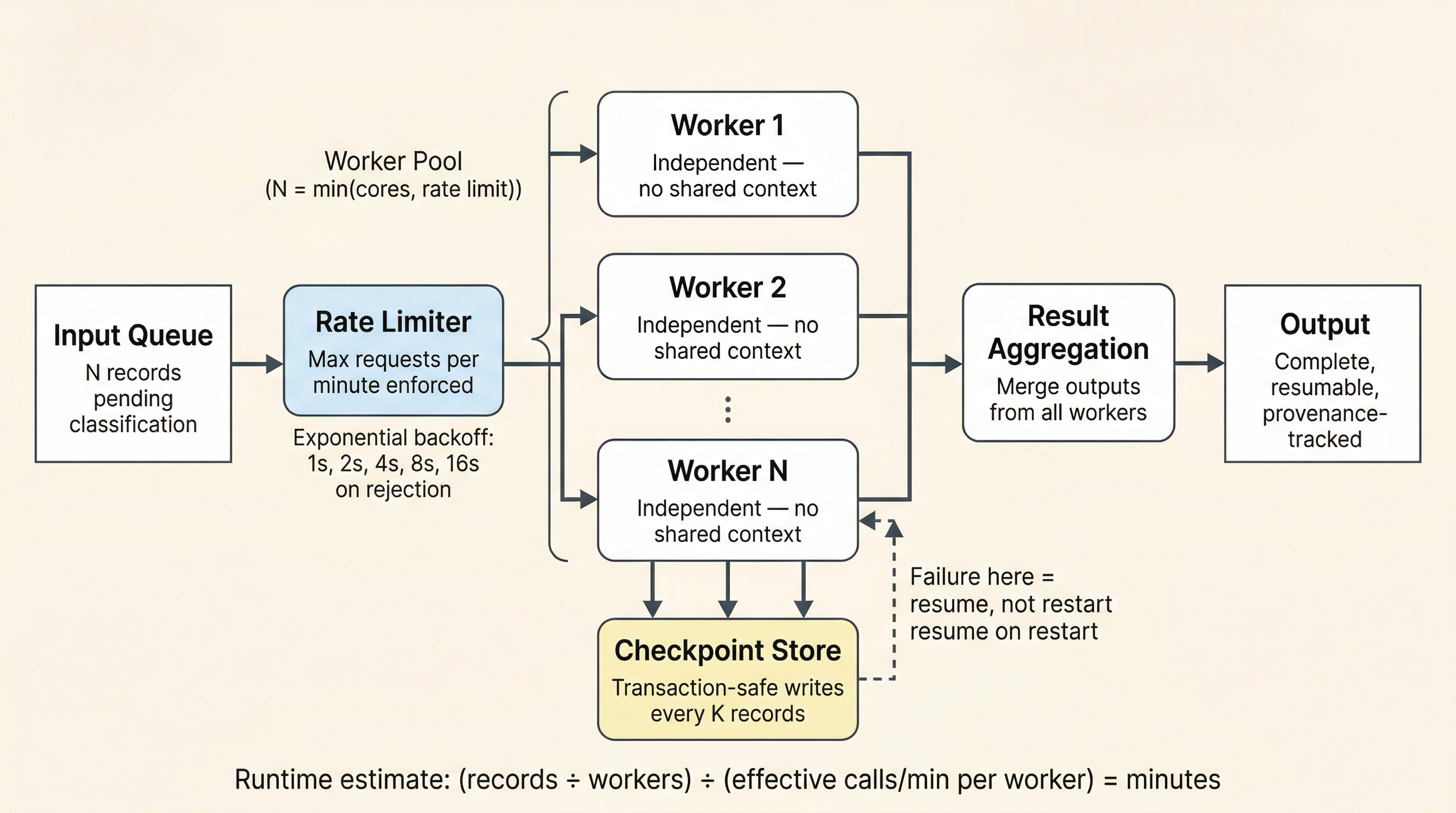
Figure 1:Parallel batch processing architecture. The rate limiter governs throughput against provider constraints; exponential backoff prevents cascading failures on rejection. N independent workers process batches with no shared context. The checkpoint store enables resume-on-failure without restart. Result aggregation merges worker outputs into the final deliverable.
You are processing 50,000 records through an LLM pipeline. Your provider allows 60 requests per minute. How many parallel workers can you run? What happens when one worker’s batch fails at record 3,000: does the whole pipeline restart, or just that worker’s batch?
Model Selection as Engineering Decision
People spend weeks running comparison experiments over fractional accuracy differences between models. This is the bike-shedding trap applied to AI: burning engineering time on decisions that matter less than the time spent making them.
Simpler models earn their place by default. A smaller, cheaper model is faster to process, has higher rate limits (less resource-intensive on the provider side), and costs less per call. Unless the task demonstrably requires frontier capability, and you should need evidence rather than intuition to make that claim, the simpler model wins on every operational dimension that matters for batch processing.
The engineering time burned on marginal comparison experiments (2-3 percentage points of accuracy, 10-15% cost differences) typically costs more than the difference between the models ever would at production scale. Use available benchmarks and cost tables for a quick tradeoff analysis. Make a decision. Move on. Chapter 14 provides the full cost accounting framework.
This connects to the evaluation trap from Chapter 1. The rate of model advancement is so fast that extended comparison experiments produce obsolete conclusions. Models update silently. New contenders enter the market. If you spend six months testing five models, those models have already changed by the time you publish results. You do not have six months. Make engineering decisions with available information and design the system to absorb change.
The ensemble reframe kills bike-shedding. If two models are close in performance, the correct engineering answer is not “run more experiments to find the winner.” It is “use both.” Now you have disagreement detection, systematic bias discovery, and higher composite confidence, which is worth more than the marginal performance difference you were trying to measure. Without the second model, weird biases and systematic blind spots remain invisible. They only surface in disagreement patterns. This connects back to Chapter 5’s thesis: multi-model is the baseline, single-model needs justification.
Two models score 91% and 89% on your classification benchmark. You estimate it would take three weeks of testing to determine if the difference is meaningful. What is the engineering decision?
Design for Change, Not for the Current Model
The model is a replaceable component. The architecture is the durable investment.
Swap-ready interfaces. The pipeline should call models through an abstraction layer: configuration-driven model selection, not hardcoded model names in source code. When you need to swap a model (and you will), it is a config change, not a code rewrite.
Versioned configurations. Every pipeline run records which model, which version, which parameters were used. This is provenance (connects to Chapter 10) and it is also practical: when results change between runs, you need to know whether you changed something or the provider did.
State has shape; match your storage to it. Versioned configurations, run logs, and parameter snapshots are tabular. A relational database or structured config files handle them well. But pipeline state that involves typed relationships between entities, artifacts that depend on other artifacts, decisions that supersede prior decisions, evidence chains that connect claims to their sources, is graph-shaped. Forcing graph-shaped state into foreign keys and JOIN tables loses the relationship structure that makes provenance auditable and impact analysis tractable. The design choice is not “relational or graph.” It is “what shape is this state?” Tabular state stays tabular. Relationship-rich state gets a relationship-aware data model. Chapter 10 provides the implementation guidance; the point here is that the choice is driven by state shape, not by technology preference.
Model turnover is the steady state. Models deprecate. APIs change. New options appear. Pricing shifts. If your pipeline breaks when the model changes, you designed for a moment, not for a system. Design for model turnover as a normal operating condition, not as an exception.
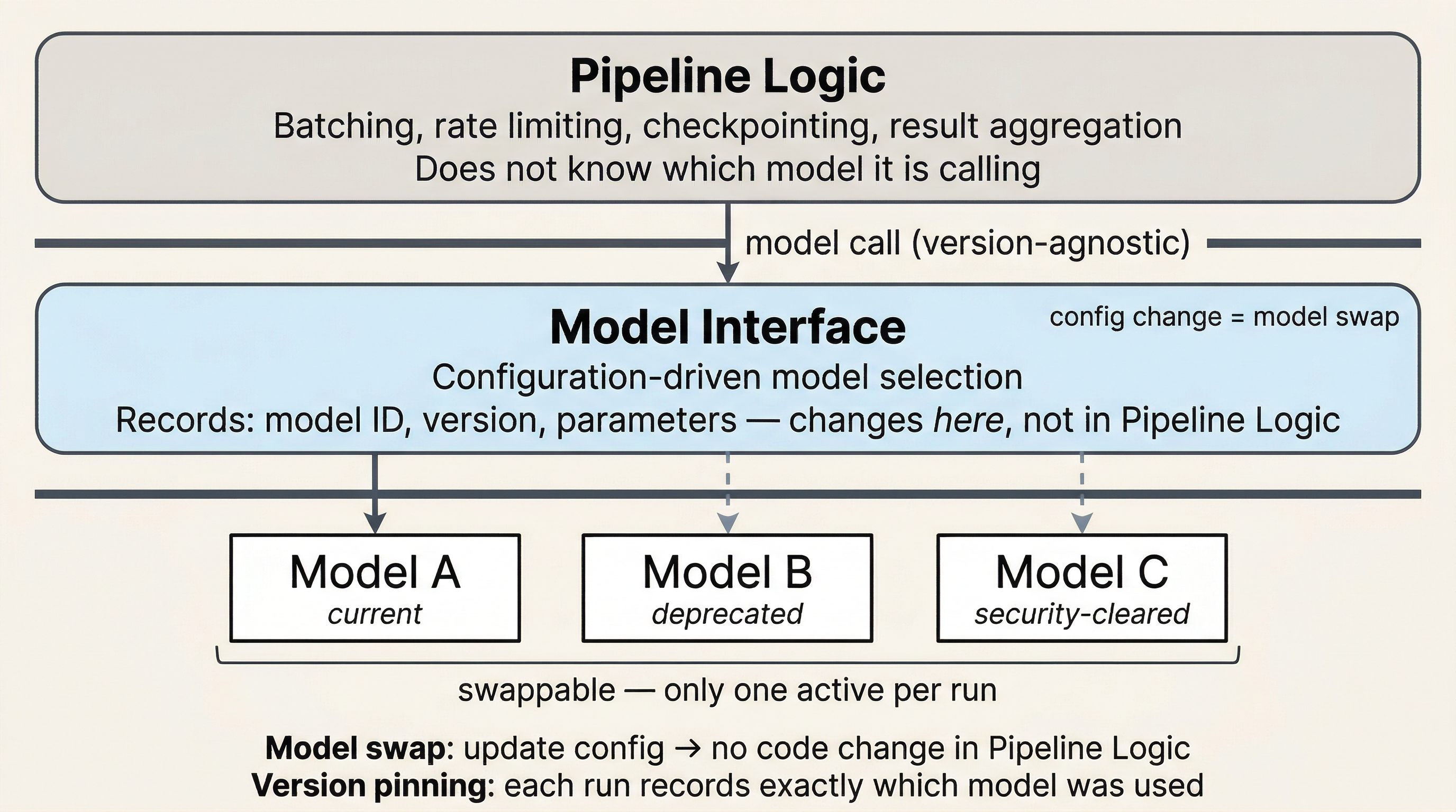
Figure 2:Model abstraction layer. Pipeline logic calls through a configuration-driven model interface that knows nothing about the specific model underneath. When the model changes, only the configuration changes. All pipeline logic, rate limiting, checkpointing, and result handling remains unchanged. Each run records the exact model version used.
Pike’s Rules Applied to Pipeline Design
Rob Pike’s five rules from Notes on Programming in C Pike, 1989 are engineering wisdom that maps directly to LLM pipeline design:
Bottlenecks surprise you. Profile your pipeline before optimizing. The bottleneck may be JSON parsing, file I/O, or rate-limit backoff sleep time, not the LLM inference itself. Do not assume. In the Concept Mapper pipeline, 40% of runtime in one workflow was spent parsing structured JSON output, not waiting for the LLM.
Measure before tuning. Instrument first, optimize second. If you are not measuring, you are guessing. This connects to Chapter 8’s evaluation-by-design thesis. At minimum, log response time, token count, and error type for every API call.
Fancy algorithms are slow when N is small, but design as if N will be large. For federal statistics, invert Pike’s caution. If the method works, it will be applied at scale. The Concept Mapper processed approximately 7,000 questions as a proof of concept, but nothing in the pipeline is hardcoded to 7,000. The architecture holds at 70,000 or 700,000.
Fancy algorithms are buggier than simple ones. Use simple data structures. Config-driven pipelines with flat JSON schemas over clever object hierarchies. Complexity is where bugs hide.
Data dominates. Get your schemas right and the pipeline design follows. This connects directly to Chapter 2’s argument for adopting existing domain frameworks Fortier et al., 2011Wolf et al., 2016 as structured output schemas rather than inventing your own.
Normalize formats at the gate. Raw document formats, PDF, DOCX, HTML, scanned images, are unfit for direct LLM consumption. A pipeline that feeds raw PDF bytes into a prompt is conflating two problems: format interpretation and content analysis. Separate them. The first stage of any pipeline that ingests documents should convert everything to a canonical text format (clean Markdown or plain text with preserved structure) before any LLM processes the content. This is infrastructure, not a prompt concern. The LLM’s token budget should be spent on reasoning about content, not on parsing layout artifacts, decoding table structures from positional whitespace, or interpreting OCR noise. Format normalization also makes your pipeline format-agnostic downstream: once everything is canonical text, the classification, extraction, or analysis stages do not need to know whether the source was a PDF, a spreadsheet, or a web page. The conversion step is deterministic (or nearly so), testable independently of the LLM, and cacheable. Build it once, validate it against your specific document types, and every downstream stage benefits.
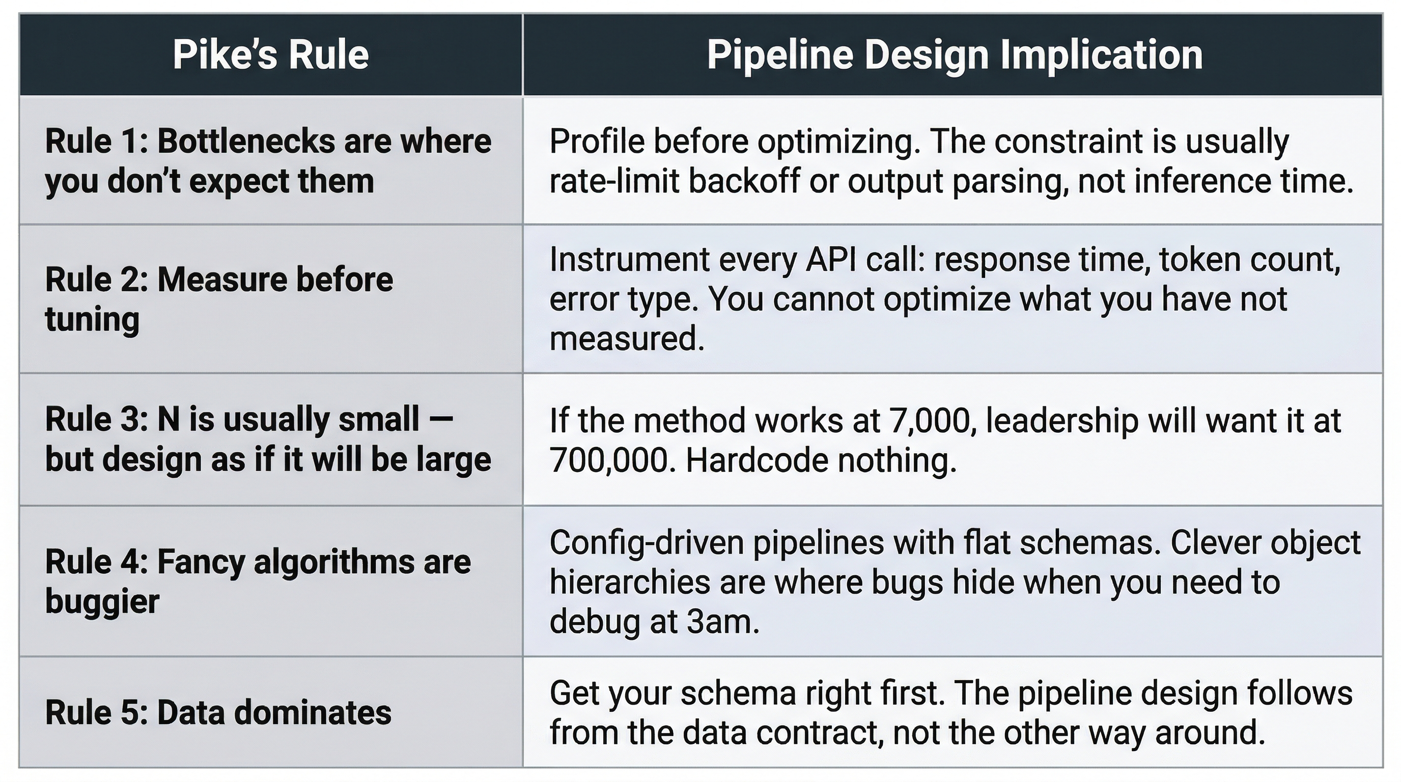
Figure 3:Pike’s five rules mapped to LLM pipeline design. Each rule surfaces a different class of engineering mistake: unverified assumptions about bottlenecks, premature optimization, failure to design for scale, hidden complexity, and schema-first design. The rules are diagnostic, not prescriptive.
Pike’s rules provide the diagnostic lens. The next question is whether your design holds when the problem gets bigger.
Design for Scale from Day One
People who design for their current small dataset build systems that only work small. When the method proves itself and leadership says “do this for all surveys” or “do this cross-agency,” the pipeline collapses because batch sizes were hardcoded, schemas were dataset-specific, and the worker pool was tuned to one machine.
Design the pipeline as a machine, not a one-off script. No hardcoded batch sizes or dataset-specific logic. Worker counts, schemas, and model selections as configuration parameters. Checkpoint and resume that works at any scale. The architecture should be indifferent to whether N is 100 or 100,000.
The compounding loop. Better pipeline infrastructure produces more productive development, which frees time to improve infrastructure, which compounds. Investing in reusable, well-designed batch processing infrastructure pays dividends on every subsequent workflow. The alternative, rebuilding rate limiting, backoff, checkpointing, and parallel dispatch for every new project, is a tax on every new initiative.
A pipeline hardcoded to one survey’s schema fails the moment a second survey uses different field names for the same concept. A pipeline hardcoded to 6 workers fails when the provider changes rate limits.
Your pipeline processes 7,000 questions successfully. Leadership says “now do this for all 47 surveys, every quarter.” What breaks first: your batch sizes, your schema definitions, your checkpoint intervals, or your rate limit budget? What would you need to change in zero of these to handle the scale increase?
The Infrastructure Reinvention Problem
Every new workflow in the Concept Mapper required rebuilding the same infrastructure: rate limiting, backoff, checkpointing, parallel dispatch. The AI coding partner would rebuild from scratch despite being given reference implementations, ignoring configuration files, inventing nonexistent model names, rewriting debugged infrastructure with its own patterns.
This is the stochastic tax (Chapter 1 introduced the concept for inference; here it applies to development itself) applied to the development process, not just the inference process. Your development tool is itself stochastic, and it introduces its own variance into the infrastructure it builds. Reusable pipeline infrastructure is an asset. Rebuilding it per-workflow is waste.
The solution is config-driven, importable infrastructure modules: rate limiting, backoff, checkpointing, and parallel dispatch as shared components, not as code that gets rewritten for every project. Chapter 7 provides the architectural pattern. Chapter 11 addresses the meta-level challenge: when your development tool is itself an LLM, the infrastructure reinvention problem is a structural feature of the development process, not a one-time mistake.
Thought Experiment
Design a classification pipeline that must survive three model swaps in 18 months without architectural rework. Your provider deprecates Model A six months after launch. A new market entrant offers Model B at half the cost with comparable accuracy. Your agency’s security review clears Model C but not Model B.
At each transition: what changes? What does not? What would break in a pipeline designed around a specific model rather than around a model interface?
Parallel pipelines create throughput. But throughput creates a new problem: what happens when something fails at record 30,000 of 50,000? Do you restart from zero? Chapter 7 treats checkpoints, failures, and recovery: the engineering discipline that makes long-running pipelines survivable.
- Webb, B. (2026). AI-Assisted Federal Survey Harmonization: Cross-Survey Integration Analysis of 47 Census Bureau Demographic Surveys. Draft working paper. https://github.com/brockwebb/federal-survey-concept-mapper
- Pike, R. (1989). Notes on Programming in C. Bell Labs internal document. https://www.lysator.liu.se/c/pikestyle.html
- Fortier, I., Doiron, D., Little, J., & others. (2011). Is Rigorous Retrospective Harmonization Possible? Application of the DataSHaPER Approach Across 53 Large Studies. International Journal of Epidemiology, 40(5), 1314–1328. 10.1093/ije/dyr106
- Wolf, C., Schneider, S. L., Behr, D., & Joye, D. (2016). Harmonizing Survey Questions Between Cultures and Over Time. In C. Wolf, D. Joye, T. W. Smith, & Y. Fu (Eds.), The SAGE Handbook of Survey Methodology (pp. 502–524). SAGE.