The Code Says 999999
A respondent self-reported their NAICS code as 999999. Their free-text business description says “I fix toilets and sinks in people’s houses.” A human coder would read the description, look up the plumbing contractor code (238220), and fix it. An LLM can do the same thing. But you have 200,000 records with bad codes, and you need to verify 200,000 corrections.
This is not classification in the Chapter 2 sense. In Chapter 2, the input was well-formed: clear survey questions mapped to a structured taxonomy. Here, the input itself is the problem. Wrong codes, ambiguous descriptions, inconsistent formats, data arriving in five different file layouts. The LLM’s job is not to classify clean input. It is to interpret messy human input and map it to structured output.
The design challenge is verification at scale. An LLM that proposes a “corrected” NAICS code with high confidence is performing what Chapter 4 will call confidence laundering if there is no evidence chain for why that correction is right. The dual-model patterns from Chapter 2 apply, but the error modes are different because the input quality is worse. When the input is noisy, single-model confidence is even less trustworthy than it was for clean classification.
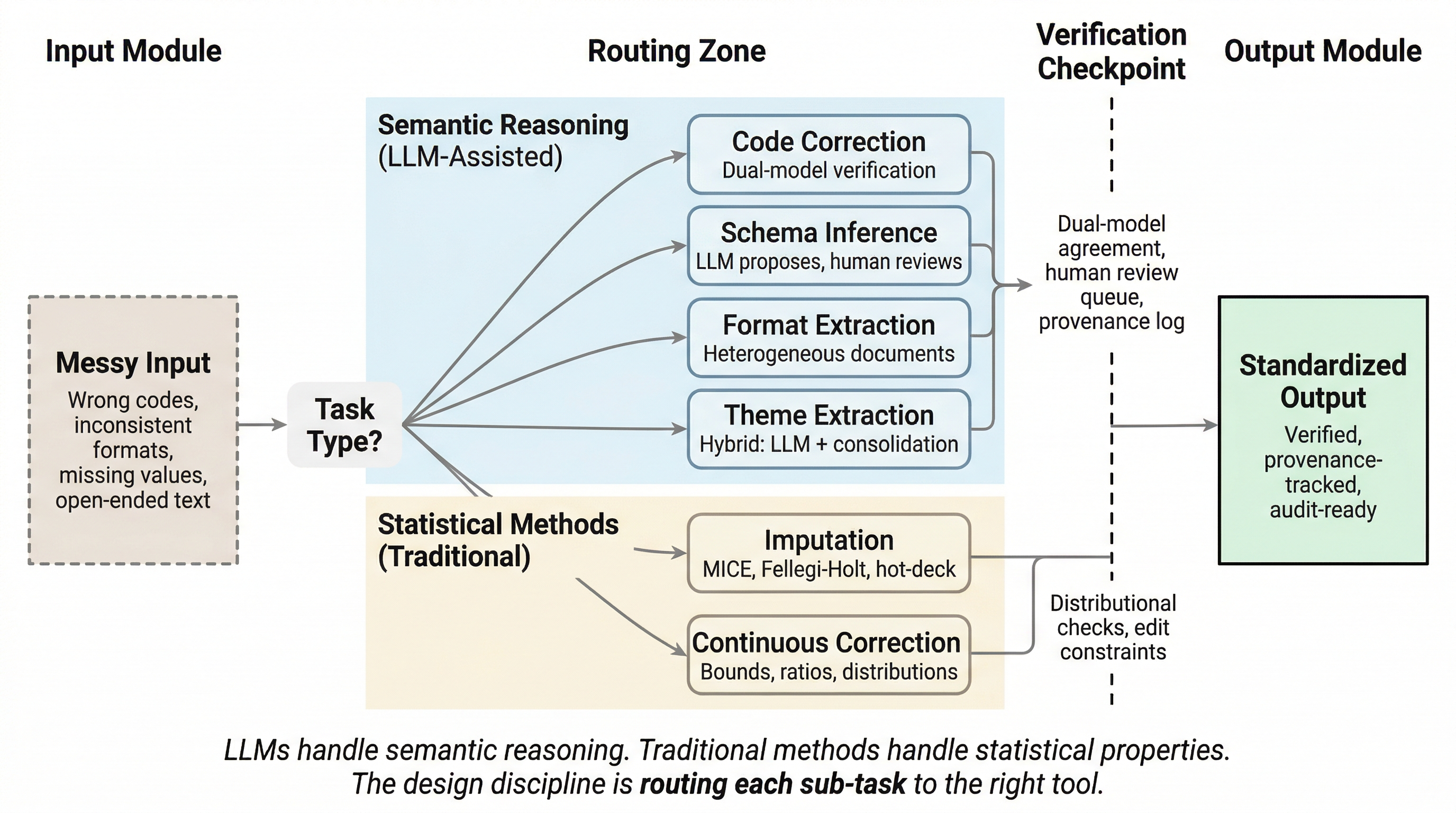
Figure 1:Data quality pipeline routing. Semantic reasoning tasks route to LLM-assisted methods with dual-model verification; statistical tasks route to traditional methods with distributional checks. The design discipline is matching each sub-task to the right tool.
Response Code Correction
This is the core use case. Respondents provide business descriptions and job titles that must be classified into NAICS, SOC, NAPCS, and other coding systems. The resulting codes are often wrong. Sometimes wildly wrong: a restaurant coded as a hospital. Sometimes plausibly wrong: a general contractor coded as a specialty trade contractor. Classification error is well-documented, especially at detailed coding levels where agreement between independent coding methods drops substantially (Buckner-Petty et al., 2019). LLMs can read the free-text description alongside the assigned code and propose corrections.
This is classification (Chapter 2 patterns apply) but with dirty input. The error modes are different from clean-input classification in important ways. The respondent’s description might itself be ambiguous (“I do construction work” could be half a dozen NAICS codes), incomplete (“I work with computers”), or wrong (the description does not match what the business actually does). The LLM is reasoning over two unreliable signals: a code that is probably wrong and a description that may not be right either.
Dual-model cross-validation matters even more here than it did in Chapter 2. When input noise makes single-model confidence less reliable, the disagreement signal between two independent models becomes the primary quality indicator. If both models independently read “I fix toilets and sinks” and propose 238220 (Plumbing, Heating, and Air-Conditioning Contractors), you have meaningful convergence. If they disagree, the disagreement tells you something about the ambiguity of the input, not just about the models.
Confidence routing follows the same pattern as Chapter 2: high-confidence corrections auto-accept, low-confidence corrections route to the human review queue. But the thresholds may need to be different. Input noise means the pipeline will produce more low-confidence cases, and the fraction requiring human review will be larger than for clean-input classification. Design for that. Budget the human review time alongside the API cost.
Position in the pipeline matters. Code correction happens after initial data receipt and before downstream analysis. Getting this wrong propagates silently. A bad NAICS code that passes through correction unchallenged affects industry tabulations, economic indicators, and any analysis that stratifies by industry. The error is invisible in the output file. It looks like a valid code.
You have 200,000 records with self-reported NAICS codes. A quality audit of a 1% sample suggests 25% of codes are wrong. How do you estimate the total correction workload before running the full pipeline? What is the cost of not correcting them?
The Fine-Tuning Cost Trap
Some agencies are using machine learning and language model techniques for NAICS, NAPCS, and occupation coding. The Census Bureau’s SINCT system for NAPCS coding reduced write-in responses by 78% in the 2022 Economic Census (U.S. Census Bureau, 2024), and a 2025 modernization effort applied LLM embeddings and fine-tuning to improve ACS occupation and industry autocoding (Reveal Global Consulting, 2025). Fine-tuning is a legitimate approach, and in specific circumstances it is the right one. But teams that go down this path frequently underestimate the total cost relative to the API alternative.
The comparison most teams skip. Fine-tuning requires training data curation (who labels the training set, and how do you know the labels are right?), compute for training (GPU time, cloud or on-premises), an evaluation harness (you need to measure whether the fine-tuned model is better than what you had), retraining when the classification system updates (NAICS revisions, SOC updates), model hosting and serving infrastructure, MLOps overhead for all of the above, and staff expertise to manage the full lifecycle. The API approach requires prompt engineering, a dual-model verification pipeline (Chapter 2 patterns), and API costs per call. The cost comparison is conditional. At lower or moderate utilization, API access is operationally simpler and usually cheaper. Fine-tuning and self-hosting become cost-effective only when throughput is high, the workload is stable enough to absorb GPU and MLOps overhead, and the use case is mature enough to justify the engineering investment. The mistake most teams make is accounting for the per-call API cost while ignoring the human engineering cost of the fine-tuning pipeline: training data curation, evaluation harness development, retraining when classification systems update, model hosting, and staff expertise to manage the lifecycle. As a rough starting point: practitioner analyses suggest that below approximately $50,000 per year in projected API spend, the API path is almost always preferable. Above that threshold, the comparison becomes genuinely conditional on utilization stability, MLOps maturity, and whether the workload justifies dedicated infrastructure. Chapter 14 provides a cost accounting framework that makes this comparison rigorous.
When fine-tuning is the right call. Be honest about the cases where it earns its place. Data sensitivity that creates significant legal barriers to cloud API access: Title 13 data, Confidential Information Protection and Statistical Efficiency Act (CIPSEA)-protected microdata, and other data with legal restrictions on transmission to parties outside the agency’s authorized workforce. Latency requirements for real-time coding at production scale where API round-trip time is a binding constraint. Offline deployment requirements where network access is unavailable or unreliable. But even in these cases, the institutional deployment tax from Chapter 13 applies: finding the budget, navigating security review, procuring and installing hardware, getting priority in the infrastructure queue, setup and staff learning, quality benchmarking against the existing process. In practice, this takes 6 to 18 months before you process a single production record, where the shorter end assumes an existing authorization or ATO already covers the use case; new authorizations typically run 12 months or longer. Even the policy compliance path alone has multi-month lead times: OMB’s 2025 AI acquisition memo (Office of Management and Budget, 2025) establishes a 180-day compliance window for new contracts, with agencies required to update internal acquisition procedures within approximately eight months of issuance.
The uncomfortable truth. If institutional constraints block API access and the fine-tuning/local deployment path takes 18 months, practitioners are stuck with traditional NLP (bag of words, regex, rule-based systems) that everyone knows is inferior for this task. The design discipline here is making the cost and timeline comparison explicit so leadership can make an informed access decision. Connect this to Chapter 12 (security controls as enabling, not prohibitive) and Chapter 13 (governance that prevents delivery is governance failure).
If you are going down the local deployment path, do not wait for the hardware to start learning. Build your pipeline, evaluation harness, and quality benchmarks against public data or synthetic data now, before the procurement clears, before the GPU arrives, before the security review finishes. Use public NAICS descriptions, synthetic respondent data, or any non-restricted dataset that exercises the same classification logic. When the infrastructure finally arrives, you should be validating a proven pipeline against production data, not writing your first prompt. That procurement and security timeline is pipeline development time you can use in parallel, if you plan for it.
On small language models. The SLM landscape is evolving fast. Models that are marginal today may be substantially more capable in 12 to 18 months. The design patterns in this book, dual-model verification, confidence routing, structured arbitration, provenance tracking, apply regardless of whether the model is a frontier API model or a local quantized SLM. If you build the pipeline right, swapping the model underneath is a configuration change (Chapter 7), not a redesign. That is the entire point of model-agnostic architecture.
The System You Leave Behind
Everything in this chapter so far addresses the pipeline builder’s question: which tool handles which sub-task? There is a second question that matters just as much: what happens to this system after you ship it?
Five engineering concerns shape that answer.
Supportability. Can someone who did not build this pipeline keep it running? If the person who wrote the prompts leaves, can the next person debug a misclassification? A fine-tuned model is a black box that requires ML engineering expertise to retrain. An API-based pipeline with well-documented prompts, clear routing logic, and structured evaluation harnesses is something a competent data scientist can pick up and maintain. Design for the team you have, not the team you wish you had.
Maintainability. Classification systems change. NAICS revises. SOC updates. The taxonomy underneath your pipeline shifts, and every component that touches it needs to respond. For a fine-tuned model, that means retraining: new labels, new training data, new evaluation pass. For an API-based pipeline, it means updating the reference schema and re-running your golden test set (Chapter 8). For traditional lookup tables, it means a file swap. These are fundamentally different maintenance profiles, and the cheapest one to build is rarely the cheapest one to maintain.
Opportunity cost. Every hour spent tuning prompt temperature, chasing a half-percent accuracy improvement, or debugging a model’s edge-case behavior is an hour not spent processing data, building evaluation infrastructure, or shipping something that works. The enemy of deployed is perfected. Get the pipeline to “good enough, verified, and auditable,” then move on. You can iterate later with evidence from production, which is worth more than any amount of pre-deployment tinkering.
Designing for replaceability. The model is the most volatile component in your pipeline. Models get deprecated, pricing changes, new versions behave differently, vendors exit markets. If swapping the model underneath requires a redesign, you have coupled your architecture to a vendor’s release schedule. This is the model-agnostic architecture argument from the SLM discussion above, but stated as an engineering imperative: the model is a configuration parameter, not a load-bearing wall. Build accordingly.
The virtue of boring tools. Traditional methods do not hallucinate. Multiple Imputation by Chained Equations (MICE) does not confabulate. Hot-deck imputation does not have a training data cutoff. Bag-of-words does not drift between API versions. For the parts of your pipeline where steady, reproducible, predictable behavior is the requirement, the “inferior” tool is the superior design choice. Boring is a feature when the alternative is exciting and wrong.
These five concerns are not separate from the routing decision in this chapter’s opening figure. They are the routing decision, viewed from the perspective of the system owner rather than the system builder. When you choose between an LLM-assisted path and a traditional method, you are also choosing a maintenance profile, a supportability requirement, and an opportunity cost. Make that choice explicitly.
Schema Inference and Data Combination
Data arrives from disparate sources with different structures. CSV files with different headers. Excel workbooks with different column names. Databases with different schemas. The task: combine them into a unified target schema.
Consider a concrete case. Three surveys measure household income. Survey A has a column called household_income containing annual pre-tax values in dollars. Survey B has hh_inc containing monthly post-tax values in cents. Survey C has income_band containing categorical ranges (“$25,000-$49,999”). A human analyst looking at all three immediately spots three problems: the names differ, the units differ, and one source is categorical while the others are continuous. An LLM looking at the column names and a sample of values can spot the first two problems. It will likely miss the third, or worse, propose a mapping that silently converts categorical ranges to midpoint values without flagging the loss of information.
LLMs can read source schemas and propose mappings: auto-generate a target schema from the union of source fields, propose join keys and crosswalks between fields, identify semantic equivalences. Experimental evaluations of LLM-based schema matching confirm that models can identify semantic correspondences between columns, including cases where names are abbreviated or use domain-specific conventions. But performance depends strongly on the scope and context provided: N-to-M mappings are consistently the weakest case, and too much or too little schema context degrades matching quality. The framing from schema matching research is instructive: LLMs assist data engineers rather than replace them (Parciak et al., 2024). Recent work on agentic data harmonization takes this further, combining LLM-based reasoning with interactive human review and reusable harmonization primitives, so the human can inspect, correct, and approve each proposed mapping before it propagates downstream (Santos et al., 2025).
The schema proposal is a draft, not a final product. Human review of the proposed schema is essential, and the review must go deeper than checking whether the column names match. Semantic equivalences can be wrong in ways that are invisible at the schema level. “Income” in two different surveys may measure different constructs: gross versus net, individual versus household, annual versus monthly. The LLM is pattern-matching on field names and sample values, not reasoning about the construct definitions behind the data. This is exactly the kind of semantic gap that Chapter 8’s evaluation framework addresses, or the kind of structured expert judgment that can be delivered through system-level context (Webb, 2026).
The data harmonization literature provides a useful framework for evaluating LLM-proposed mappings. Not all mappings are equal. The retrospective harmonization literature distinguishes complete harmonization (source maps directly to target), partial harmonization (mapping requires transformation that loses information), and impossible harmonization (source cannot support the target construct) (Fortier et al., 2017). The LLM will propose a mapping for every field. It will not tell you which mappings lose information and which are impossible. That classification requires domain knowledge that the model does not have.
Two datasets both have a column called “employment_status.” Survey A codes it as 1=employed, 2=unemployed, 3=not in labor force. Survey B codes it as full-time, part-time, unemployed, retired, student, disabled, other. An LLM proposes mapping both to a unified schema. What information is lost? What crosswalk assumptions are you making? How do you document those assumptions so that downstream analysts know what they are working with?
Log the schema mapping decisions. When someone asks six months later why Field A was joined to Field B, the evidence chain exists (Chapter 10). This is a high-value, low-risk LLM application: the LLM proposes, the human reviews, the cost of the proposal is trivial, and the cost of getting it wrong is caught at review before it propagates. This is also the working principle “Reuse data before collecting more” applied to schema design: established harmonization frameworks and controlled vocabularies are reusable infrastructure. Building a new taxonomy when a usable one already exists is waste.
Format Extraction and Standardization
The “data arrived in five different formats” problem. A quarterly collection of establishment reports arrives as: three Excel workbooks with slightly different column orders, a batch of PDFs generated from a legacy system, and a folder of plain-text exports from a web form. The data content is similar, but the structure, layout, and encoding differ in every case. The task: extract the information and map it into a single target schema.
This is the universal parser use case, but the advantage is conditional. LLMs handle format diversity better than rule-based systems when documents vary widely in structure, because they interpret structure from context rather than requiring explicit parsing rules for each format. Recent benchmarking of document extraction methods confirms that LLM-based evaluation correlates better with human judgment than rule-based similarity metrics for semantically complex tables (Horn & Keuper, 2026). But rule-based and zonal OCR parsers remain superior for fixed, repetitive layouts where deterministic throughput matters more than semantic flexibility.
The design pattern is hybrid, and the routing decision matters. If you receive 10,000 PDFs that all use the same template (same field positions, same structure, same layout version), a rule-based parser with zonal OCR will be faster, cheaper, and more deterministic than an LLM. If you receive 10,000 PDFs generated by 47 different legacy systems with different layouts, column orders, and header conventions, an LLM-assisted extraction pipeline will handle the variance that a rule-based parser cannot. Most real collections fall somewhere in between: a core of stable templates with a long tail of variants. Design for both.
Define the target schema first. This is the config-driven pattern from Chapter 7: the LLM maps to the schema, it does not invent one. The schema is the contract. It lives in configuration. It is versioned. The LLM is a tool for mapping diverse inputs to that contract, not for deciding what the contract should be.
Extraction errors on structured data are different from extraction errors on unstructured data, and the detection methods differ accordingly. For structured data (tables, forms with labeled fields), automated schema validation catches most errors: did the extracted value land in the right column? Does it pass type and range checks? For unstructured data (narrative text, free-form descriptions), misinterpretation of content is the primary risk, and human review of a stratified sample is usually necessary. The stratification should oversample the long tail: the edge cases where format variance is highest are where extraction errors concentrate.
This is typically a one-time or periodic task (ingesting a new data source), not a continuous production pipeline. The cost and speed tradeoffs are different from the code correction use case: you optimize for correctness and completeness, not for throughput. When extraction is periodic, invest the review time upfront to validate the pipeline against the specific format variants you encounter. The validation pays for itself in every subsequent run.
Semantic Analysis of Open-Ended Responses
Public comments, free-text survey fields, open-ended response data. Not classification into a fixed taxonomy (Chapter 2) but interpretation, summarization, theme extraction.
This is where LLMs have a genuine advantage, but the boundary is more nuanced than it first appears. LLMs are stronger for keyword extraction and topic naming when you want semantic grouping from short, messy, or highly varied responses, because the model can infer latent meaning rather than just count repeated terms. Traditional topic models remain better when you need reproducible, corpus-level structure and simpler interpretability, or when you need a fixed coding scheme tracked consistently over time. Comparative studies show that different LLMs vary substantially in diversity versus relevance of extracted topics, which matters when your survey analysis needs stable categories rather than creative labels. In practice, the most effective pattern is often hybrid: LLMs generate candidate keywords or topic labels, then a human or rule layer consolidates them for downstream analysis.
But theme extraction is inherently subjective. Two models may extract different themes from the same corpus. This is the dual-model disagreement signal from Chapter 2: disagreement on themes is information about the ambiguity of the input, not error. When two models converge on the same themes independently, you have meaningful signal. When they diverge, the divergence tells you which themes are robust and which are artifacts of a particular model’s perspective.
Provenance matters. Which responses contributed to which themes? Can you trace a summary back to the source responses that generated it? Chapter 10’s provenance requirements apply: the theme extraction output should be traceable to the input that produced it, the model that generated it, and the prompt that framed the task.
The evaluation trap from Chapter 8 applies directly: how do you evaluate whether theme extraction is “correct” when there is no ground truth? The answer is the same as Chapter 8’s thesis: build the evaluation instrument alongside the extraction pipeline. Define what “good” theme extraction means for your domain (coverage, specificity, faithfulness to source), and evaluate against those criteria.
Where Traditional Methods Still Win
Knowing where not to use LLMs is as important as knowing where to use them. The boundary is the design discipline.
Imputation of missing values. MICE (Buuren & Groothuis-Oudshoorn, 2011), hot-deck, Fellegi-Holt (Fellegi & Holt, 1976), and other established imputation methods preserve distributional properties, respect survey design effects (weights, clustering, stratification), and are theoretically well-understood. LLMs do not maintain distributional properties and have no concept of survey design. They will impute a plausible-looking value that has no relationship to the distribution of the variable in the population. Empirical evidence confirms this: LLM-based imputation can approximate highly polarized toplines but struggles with less polarized questions and subgroup estimates, with mean absolute subgroup errors exceeding 10 percentage points Morris, 2025. Adding extra anchors or chain-of-thought prompting did not reliably improve population totals. Survey weights do not solve the core problem, because weighted estimates still depend on the model’s ability to represent the missing-data mechanism and the joint distribution of responses. For continuous variables and for maintaining statistical properties, traditional methods are not just adequate; they are superior.
Continuous variable correction. When the value is numeric and the correction needs to preserve distributional properties, statistical methods outperform LLMs. An edit/imputation system that enforces ratio constraints, bounds checking, and distributional consistency is doing work that a language model is structurally unable to do.
Tian et al. (2025) compared LLM imputation against MICE and KNN on categorical variables in a real 2024 U.S. election survey with induced nonresponse. Llama 2 13B with few-shot prompting achieved mean F1 of 0.61 to 0.67 across three question sets, exceeding MICE (0.50 to 0.61) on two of three datasets and tying it on the third, at 40 times the computational cost. The advantage was strongest on polarized items where response patterns cluster clearly; on less polarized questions, the LLM’s edge narrowed or disappeared. Even in the best case for LLMs, the cost-performance tradeoff is narrow, and it only favors LLMs on categorical variables where the “imputation” is closer to classification (what category does this record belong to?) than to statistical estimation (what value should this variable have?). This is evidence that the boundary is real, not an endorsement of replacing established imputation methods with LLMs.
The thesis: LLMs handle the semantic reasoning parts of the data quality pipeline. Traditional methods handle the statistical parts. The design discipline is routing each sub-task to the right tool.
Thought Experiment
You receive a dataset of 500,000 business registrations with self-reported NAICS codes and free-text business descriptions. Quality audit of a sample suggests approximately 25% of NAICS codes are wrong. Design the correction pipeline:
How do you use the free-text descriptions to propose corrections? What about records with no description?
How do you decide which corrections to auto-accept versus route to human review?
How do you evaluate whether your correction pipeline is actually improving data quality, given that you do not have ground truth for most records?
At what scale does the API cost argument change? Is there a volume threshold where fine-tuning becomes cost-effective?
How would your design change if the data are Title 13, CIPSEA, or otherwise restricted by policy or statutory requirement?
Chapter 3 addressed the problem of fixing and standardizing data you already have. Chapter 4 addresses extracting structured data from unstructured sources, entity extraction, pattern detection, disclosure review, where the design challenge shifts from “correct the record” to “find the signal.” The confidence laundering risk previewed in this chapter gets its full treatment there.
- Buckner-Petty, S., Dale, A. M., & Evanoff, B. A. (2019). Efficiency of autocoding programs for converting job descriptors into Standard Occupational Classification (SOC) codes. American Journal of Industrial Medicine, 62(1), 59–68. 10.1002/ajim.22928
- U.S. Census Bureau. (2024). Machine Learning for In-Instrument Product Code Search: SINCT for NAPCS Coding. FedCASIC 2024 Conference Presentation.
- Reveal Global Consulting. (2025). ACS Autocoder Modernization: LLM Embeddings and Fine-Tuning for Occupation and Industry Coding. Technical report.
- Office of Management and Budget. (2025). Responsible Procurement of Artificial Intelligence in Government [Techreport]. Executive Office of the President.
- Parciak, M., Vandevoort, B., Neven, F., Peeters, L. M., & Vansummeren, S. (2024). Schema Matching with Large Language Models: An Experimental Study. VLDB 2024 Workshop: Tabular Data Analysis Workshop (TaDA).
- Santos, A., Garcia, A., Strubell, E., Rekatsinas, T., Li, F. T., & Altman, R. B. (2025). Interactive Data Harmonization with LLM Agents: Opportunities and Challenges. arXiv Preprint arXiv:2502.07132. https://arxiv.org/abs/2502.07132
- Webb, B. (2026). Pragmatics: Delivering Expert Judgment to AI Systems. Zenodo. 10.5281/zenodo.18913092
- Fortier, I., Raina, P., van den Heuvel, E. R., & others. (2017). Maelstrom Research Guidelines for Rigorous Retrospective Data Harmonization. International Journal of Epidemiology, 46(1), 103–115. 10.1093/ije/dyw075
- Horn, P., & Keuper, J. (2026). Benchmarking PDF Parsers on Table Extraction with LLM-based Semantic Evaluation. arXiv Preprint.
- van Buuren, S., & Groothuis-Oudshoorn, K. (2011). mice: Multivariate Imputation by Chained Equations in R. Journal of Statistical Software, 45(3), 1–67.
- Fellegi, I. P., & Holt, D. T. (1976). A Systematic Approach to Automatic Edit and Imputation. Journal of the American Statistical Association, 71(353), 17–35.
- Morris, D. (2025). The Risks of Using LLM Imputation of Survey Data to Produce “Synthetic Samples.” Verasight. https://www.verasight.io/reports/synthetic-sampling-2
- Tian, W. (Sarah), Lu, Y.-S. (Angelina), Ding, Y., & West, B. T. (2025). Comparing Large Language Models and Traditional Methods for Imputing Missing Survey Responses in a 2024 U.S. Presidential Election Survey. AAPOR 2025 Annual Conference.